Defined Duration Strategy

LIKE many strategies in this book, the Defined Duration Strategy grew out of personal experiences. In this case, my personal experience. It’s designed to solve for the ultimate problem in life – time.

Before I had children, my asset allocation was typically aggressive and long-term oriented. When it came to financial planning, my life was simple as it was just me, my wife, the most incredible Aussie Shepherd that ever existed and a flock of chickens.^* I had one primary time horizon to consider and that was the time horizon my wife and I would navigate together. We both earned good incomes and so our portfolio had a long-term time horizon and we could afford to be very aggressive.

We had our first daughter just weeks before the Covid crash of 2020, and our portfolio fell significantly. I wasn’t sleeping, the news was saying millions could die, and to top it off, my mother-in-law got trapped with us after the travel ban. My morning routine consisted of crying in the shower for 30 minutes before screaming into a sock for another 10.^* Although we never realized the losses in the downturn, it was the first time in my life where my asset allocation felt irresponsible. After all, I now had a whole new time horizon to worry about – my daughter’s time horizon.

I had spent much of my career helping other investors navigate difficult timelines, especially around retirement. But this was the first time where I felt like I was not well equipped to navigate a financial plan with multiple time horizons. Ironically, I’d spent the past 15 years studying pension funds and banks – institutions that are experts at managing time-based assets and liabilities. If you’re familiar with my research, you probably know banking is a topic I’ve spent far too much time writing about. On the surface, banks are boring – but underneath, their portfolios are often intricate exercises in timing.

When banks allocate assets they have an inherent asset-liability mismatch. In other words, banks typically borrow short and lend long, which can leave them with the difficult portfolio management problem of trying to smoothly manage deposit outflows while holding a portfolio of longer-duration assets as most loans are. Banks have a temporal conundrum in their balance sheets that forces them to be overly aware of any mismatch that could create capital constraints.

NOT SO FUN SIDE NOTE

When I began to think about this in more detail it occurred to me that banks face the same problem that every investor in the world does. We all have an inherent asset-liability mismatch. We earn income in the short term and use it to manage near-term expenses. At the same time, we hold long-term assets like stocks and bonds that produce uncertain returns – and rely on those assets to fund future, unpredictable liabilities like weddings, retirement, and other major life events.

I began to wonder if the way we allocate assets is fundamentally incomplete. I’d been trained to perform risk profiles for clients and then choose instruments to diversify across asset classes. But investors aren’t just seeking diversification of instruments – they’re looking for diversification across instruments and time. And in the end, isn’t time what we’re really trying to manage? We shouldn’t be focused solely on beating the market or diversification of assets alone. Instead, we should aim to build financial planning-based portfolios that increase the certainty of meeting future financial needs across all the different time horizons we encounter in life.

Remember that Ken French quote: “risk is uncertainty of lifetime consumption.” Bingo. Our asset allocation should be constructed to optimize our ability to navigate future consumption.

After I stopped screaming into socks, I wrote a paper in 2022 titled “Defined Duration Investing.” The goal was to create a model for asset management that not only diversified portfolios across asset classes, but also across time horizons – so investors could better understand how specific assets align with specific financial goals in the future. For example, bond investing is incredibly clean because you know the key variables:

• A bond has a fixed time horizon.
• A bond has a fixed payout.
• A bond has a specific credit quality.

If you buy a 12-month T-bill yielding 4%, you know exactly what your asset is providing relative to any future liabilities you might incur. You know the return, the time horizon and the principal stability of the instrument over the time period.

This is why the strategy of bond laddering is so useful. If you hold one-, two-, and three-year bonds, you’ve created a laddered temporal asset allocation that gives you a nearly precise ability to understand what your future cash flows will look like.

But what if you could introduce other assets like stocks or commodities into the ladder? Then you could create a temporally allocated portfolio that included the assets that have the most temporal uncertainty. After all, we don’t really know the duration of the stock market or commodities, and it’s that uncertainty that makes them the most difficult to plan around.

The Defined Duration Strategy tries to solve this problem by quantifying the time horizon of the stock market (and any asset) to give us a better perspective of the time horizon over which those instruments can be reasonably relied upon to generate certain returns. We can then blend those assets together or match them specifically to a financial plan so that the investor aligns assets and expected liabilities. You can also apply this to William Sharpe’s “arithmetic of active management.” That is, if all investors held assets across their appropriate time horizons, they would earn higher returns by reducing frictions along the way. You can’t squeeze more yield from a 10-year bond by trading it every 10 minutes. And in fact, the more investors trade that instrument, the lower their aggregate returns will be due to the various costs of doing so.

If, on the other hand, investors held assets across their appropriate time horizons they’d earn higher average returns. In other words, the average investor who holds their assets to maturity will earn a higher after-tax and after-fee return when compared to the average investor who tries to trade that asset in an attempt to earn more than it is designed to generate across its lifetime. The Defined Duration Strategy is designed to apply appropriate time horizons to certain assets thereby helping the average investor earn higher returns by holding the assets across appropriate time horizons.

In building out the model for this approach I took a concept from Bill Bernstein. Bernstein once proposed that you could quantify the “duration” of stocks by identifying a “point of indifference” – the point at which an investor would be indifferent to a drawdown because the asset has reached a real break-even point.

For example, if the stock market were to fall 50% in a worst-case scenario but is expected to earn a 5% real return annually, the investor reaches indifference when the asset’s value recovers to a positive real return. In this case, that recovery takes 14.21 years. If you had bought global stocks at their peak in 2007 and they earned 5% real returns annually, you’d be indifferent to the GFC loss after 14.21 years. That’s the stock market’s “defined duration” – the time frame over which you can reasonably assess the asset’s performance relative to your sequence-of-returns risk and ability to plan future consumption with very high confidence.

If you recall the data from Essential Principle #8, you’ll remember that the probability of positive returns for the stock market over a 10- to 20-year period is around 90–99%. So this time horizon aligns with both historical and statistical expectations.

Admittedly, this approach is probably a bit conservative as it assumes a severe max drawdown scenario, but in investing we should plan for the worst and hope for the best. Of course, the inputs here are dynamic by design. You would have to modify the expected max drawdown and expected returns as market conditions change. And typically, as stocks decline in value, we should expect the potential max drawdown to be reduced while the expected future return increases, and vice versa.

More importantly, although we’re attempting to apply precise time horizons to instruments, we know we’re also providing a general framework for how to think about certain assets. Stocks are long-term instruments and can be thought of as being similar to a multi-decade bond that will pay an average coupon of 5% real returns if you are willing to hold it for 15–20 years. They should never be thought of as daily, monthly, or even annual instruments because they cannot mathematically distribute all their profits consistently over such brief time horizons and therefore do not generate reliable short-term returns.

This methodology also allows us to quantify the defined duration of any instrument or multi-asset strategy. For example, if we input the 60/40 Portfolio into this model and assume a max drawdown of 30% (the 2008 downturn) and expected 3% annual real returns, then the defined duration of this instrument would be approximately 12 years. This makes intuitive sense: an aggregate bond index has a defined duration of around five years, and if you blend that with an 18-year instrument (the defined duration of global stocks as of 2025), you arrive at an aggregate instrument with a defined duration that is longer than bonds but shorter than equities. As I’ve noted before, this is the beauty of the 60/40 Portfolio. It blends the long duration of equities with the shorter duration of bonds, resulting in more stable and reliable returns. But even the 60/40 needs to be thought of as a somewhat longer duration instrument because stocks skew its principal sensitivity heavily.

The most interesting conclusion from this model is that many of the “alternative” assets we’ve discussed in this book end up having characteristics that are similar to insurance. Insurance typically has a low or negative expected real return, but when triggered it generates a huge asymmetric payoff. Doesn’t that sound a lot like long-term Treasury bonds, options, gold, Trend Following, or managed futures?

As we’ve discussed throughout this book, these instruments often have highly asymmetric returns in very specific environments. T-bonds generate strong asymmetric returns in deflations, gold performs best in periods of high inflation, managed futures and Trend Following excel during market anomalies, and far out-of-the money options can produce large payoffs in extreme tail risk events. In contrast, core assets like cash, intermediate-term bonds, and stocks tend to offer more stable, broadly reliable behavior over time, making them foundational building blocks. Alternatives, on the other hand, act more like long-term insurance, providing protection when those core assets face unusual or adverse conditions.

Table 20.1 shows how the defined duration time horizons look across different instruments as of 2025.

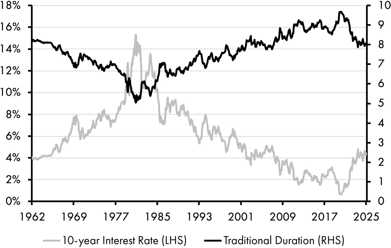
But it’s important to emphasize that durations are not static. For example, Figure 20.1 shows the traditional duration of a 10-year T-note. This is crucially important for an investor who is sensitive to price changes because it means that a lower yielding bond will not protect you as well from potential rate increases and their coinciding principal losses. A 1% yielding T-note in 2020 is vastly riskier than a 5% yielding T-note in 2025 because its starting interest rate will not protect you to the same degree from potential interest rate risk in the short term.

Table 20.1: Asset class durations (as of 2025)

This negative impact is especially harmful in bond funds like a bond aggregate where, not only has duration drifted higher and higher in recent decades, but longer duration government bonds have become an increasingly large component in the index over time, rising from 25% of the holdings in 1975 to 40% at present. This is why the bond market is one place where it makes a good deal of sense to be more active. If you simply “take what the market gives you” then you’re being fed a constant meal of low yield and long duration interest rate risk from the government, which can expose you to excess principal risk over time and lower risk-adjusted returns. This is one of several major flaws in aggregate bond funds, as they rebalance back to a cap weighting that is dominated by what the government issues.

Figure 20.1: Traditional duration of 10-year T-note

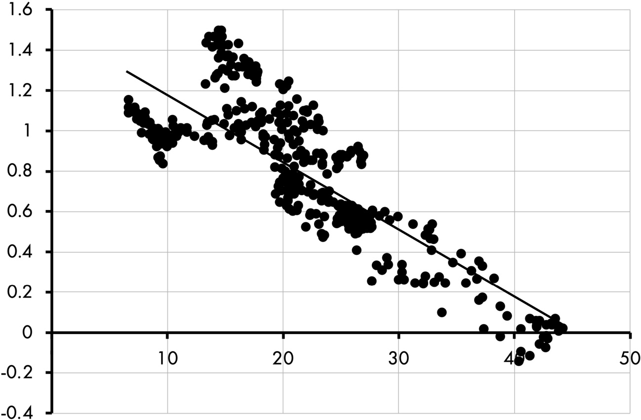
Although this evolving duration dynamic is most obvious in bonds, the same general thing happens in all markets over time as asset prices boom and bust. The bond market happens to be one of the easier places to control it because you can explicitly dial back the temporal sensitivity of the instrument. We don’t have the same luxury in the stock market where all the instruments are functionally longer in duration, however, we can still see clear evidence that indicators such as high valuations tend to correlate with lower future risk-adjusted returns, as shown in Figure 20.2. We learned in the Countercyclical Rebalancing chapter that valuations alone aren’t good short-term return predictors, but if you’re behaviorally sensitive to short-term volatility it makes sense to manage the risk around the instrument using some sort of countercyclical model.

Therefore, in multi-asset instruments (like a 60/40 stock/bond portfolio), it is sensible to control for duration risk across all instruments, assuming you’re using the instrument to create stability over a 10–12-year time horizon. That is the beauty of rebalancing back to 60/40, after all – you’re throttling the procyclical growth of the 60% slice whenever it grows above 60% exposure which helps avoid its defined duration from growing longer. Defined Duration Investing will inevitably require a certain degree of strategic rebalancing in the strategy as you’re creating specific temporal targets using some inherently uncertain temporal instruments.

Figure 20.2: CAPE versus 10-year Sharpe ratio

WHY DEFINED DURATION INVESTING WORKS

Defined Duration Investing (DDI) is a financial planning and behavioral strategy similar to what researchers have called “liability-driven investing” or “time segmentation” strategies. However, DDI goes a step further and specifically quantifies the time horizon of the assets in the portfolio to try to create greater certainty and clarity over the specific time horizons we’re targeting. Traditional bucketing strategies use vague categories like “short-term,” “medium-term” or “long-term,” and don’t measure the actual duration of each asset. Traditional liability-driven strategies are usually limited to fixed income and traditional duration metrics. DDI expands on these approaches by assigning explicit durations to all asset types – including stocks and alternatives. In doing so we create a more quantifiable and precise asset-liability matching strategy.

Recall the chart of diversification from the Essential Principles at the beginning of this book (Figure 0.3). Diversification works because we layer different assets with different return streams. DDI takes this concept a step further by not only incorporating a wide range of assets, but by intentionally layering assets with different time horizons into a planning-based framework. For example, when you buy Chevron and Exxon stock you are diversifying by reducing the single entity risk. But you’re still invested in corporations, which are inherently long-term entities. But if you add five-year Chevron and Exxon bonds into the mix then you’re not only expanding asset diversification, you’re also diversifying temporally.

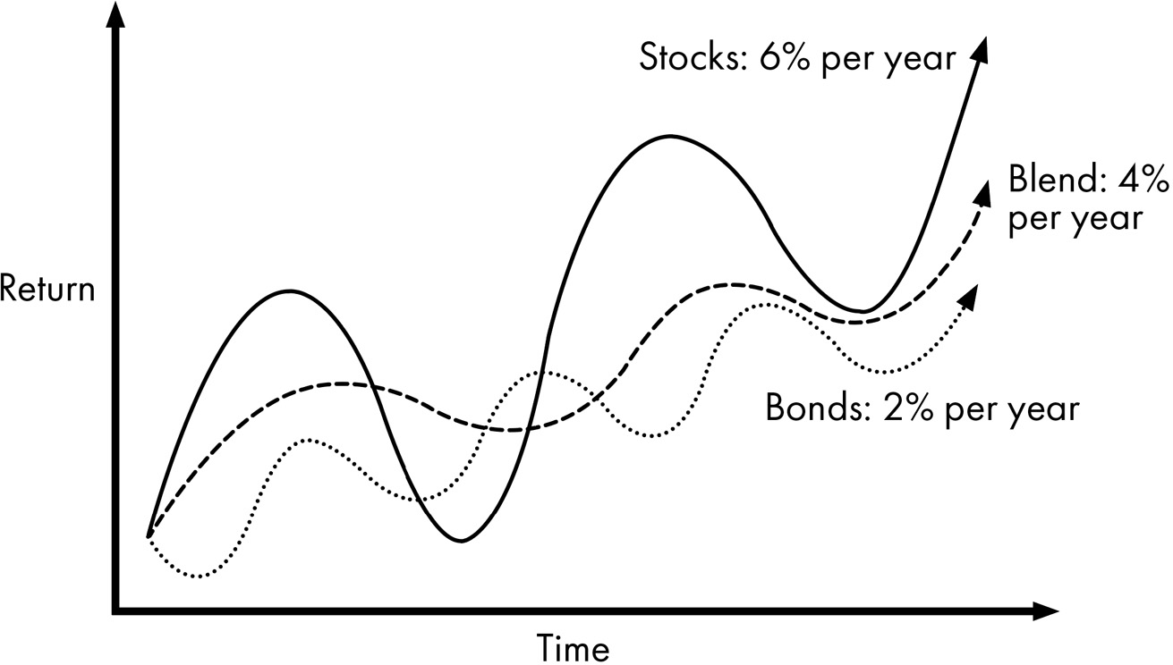
To use a clear example of why this works, you might consider a scenario where stocks are expected to generate 6% per year and bonds are expected to generate 2% per year. These are specifically different temporal instruments because the stocks will reliably generate this average return over a period of 18 years using my methodology, whereas the bonds can reliably generate their 2% return over a five-year time horizon. When you blend these two return streams, you’re creating a blended return stream that creates an expected return of 4% per year over 11 years. Figure 20.3 shows how this looks.

Figure 20.3: Why diversification of time works

As discussed further below, the strategy “works” because it starts with a financial plan and then matches assets to that financial plan to increase the certainty of cash flows around specific time horizons. The goal is to give the investor a better understanding of the way their assets align with future expected expenses and consumption needs. By quantifying the time horizon of each asset, the strategy aims to improve behavior and provide greater clarity and confidence in the financial planning process.

In my experience it’s not only a sound financial planning-based asset management strategy, but it’s a powerful behavioral tool. By clearly quantifying each portfolio component and aligning it with specific goals and time horizons, the strategy helps compartmentalize assets in a way that supports both clarity and discipline.

For example, in our exploration of the 60/40 Portfolio I referred to “homogeneous portfolio risk.” This happens when a portfolio is structured as one large, aggregated group of assets. While it may be diversified on the surface, it doesn’t provide clear visibility or access to each specific asset. So even if the 60/40 Portfolio includes cash or short-term bonds, you can’t necessarily access that liquidity when needed – unless you disaggregate the portfolio and isolate the individual components.

I’ve found that disaggregating portfolios into these very specific temporally defined buckets helps to give an investor more certainty over their portfolio and oftentimes helps them take more risk (and generate higher returns) than they might otherwise. That’s because the assets are clearly compartmentalized into specific buckets where, for example, your long-term assets are segmented into a long-term bucket that are allowed to perform in the long-term manner they’re intended to. We shouldn’t care what the long-term bucket does in the short term because we know our short-term assets are there to meet any potential short-term liquidity needs. As a result of this, if the stock market goes down significantly you can simply ignore that component knowing that you hold some percentage of your assets in T-bills or other short-term buckets that are more than enough to weather a potentially multi-year bear market in stocks.

In short, Defined Duration Investing works because it’s a financial planning-based approach to asset management that helps you build a more complete asset ladder using cash, bonds, stocks, and alternatives diversified over specific time horizons. It’s not a “beat the market” or “alpha maximizer” portfolio. It’s just a sensible asset allocation approach that helps us build temporally diversified portfolios in a quantifiable, planning-based approach.

BUILDING YOUR OWN DEFINED DURATION PORTFOLIO

Most financial planning asset allocation strategies start with an investor risk profile and then allocate assets within a diversified portfolio based primarily on behavioral tendencies and financial goals.

The Defined Duration Strategy is most effective when it begins with a comprehensive financial plan that projects your expenses and liabilities over the course of your life. Unlike traditional approaches that focus on optimizing portfolios for alpha, this strategy is rooted in planning and aims to align assets with the timing of future obligations. By identifying specific future expenses, you gain greater clarity and confidence across your time horizons. From there, you match assets to those time frames – starting with short-term liabilities and methodically building a portfolio that addresses needs across the full spectrum of your financial future.

One way to implement this approach is to think of your portfolio over five specific time horizons. I call these time horizons the five pillars of Defined Duration:

1. Short-term liquidity needs (0–3 years): Emergency fund coverage and short-term spending needs.
2. Intermediate-term liquidity needs (3–7 years): Expenses like a house down payment, weddings, childcare, or major purchases.
3. Moderate long-term needs (7–15 years): Near-retirement expenses, college tuition, and other mid-horizon planning.
4. Long-term needs (15+ years): Retirement, healthcare, and multi-generational wealth planning.
5. Insurance needs (perpetual/unknown): A flexible allocation for unpredictable risks and extreme scenarios.

Building your financial plan to cover all five of the pillars ensures coverage across every time horizon you might encounter throughout your financial life.

How much to apply to each time horizon?

I always start with short-term planning needs as that’s the bucket that we can most accurately predict. As a broad rule, think of it like this:

• 0–3 years: Allocate enough to cover at least one to three years of emergency expenses and current income gaps.
• 3–7 years: Fully fund any planned expenses in this window – such as a house down payment, weddings, or planned car purchases.
• 7–15 years: Allocate roughly 5x your annual expenses or 25% of total financial assets.
• 15+ years: Allocate about 10x your annual expenses or 50% of total financial assets (or the remaining balance not required by the first three pillars).
• Insurance: Consider allocating 5–10% of your total financial assets, depending on your personal situation and risk tolerance. This bucket is often optional, but it can be valuable for hedging extreme outcomes.

I like to think of each of these time horizons as their own organized bucket. Using the average time horizon you can distill each bucket into its own customizable temporal allocation:

• 1.5 year defined duration
• 5 year defined duration
• 10 year defined duration
• 15+ year defined duration
• Perpetual defined duration

Customizing each bucket individually can refine the matching process and further smooth sequence of return risk. The goal is to align each bucket with a specific time horizon – enabling financial plans that more effectively match assets to liabilities and hopefully avoid situations where, such as recently, intermediate bonds have been allowed to drift into longer duration and riskier instruments that create excessive principal instability. As always, if you’d like more details on how I construct and customize these portfolios, feel free to reach out to me directly at cullenroche@disciplinefunds.com.

Continuing our implementation example – if you had a portfolio of $1,000,000, an expected house down payment in the coming five years of $100,000, and annual expenses of $50,000 that were fully covered by Social Security, then you would want the following allocations:

• 0–3 years (short-term needs): $100,000 (2x annual expenses) in a custom T-bill ladder and/or cash equivalents.
• 3–7 years (intermediate-term needs): $100,000 for the home down payment, matched to a five year defined duration.
• 7–15 years (moderate long-term needs): $250,000 (5x annual expenses) matched to a 10 year defined duration.
• 15+ years (long-term growth): $450,000 or 45% (the remaining balance) of the portfolio matched to a 15+ year defined duration.
• Insurance needs (unknown time horizon): $100,000 or 10% in instruments that behave like long-term hedges – such as long-term TIPS, Treasuries, managed futures, gold, or options.

If you forgo the insurance bucket (let’s say you don’t like gold or higher-fee instruments like managed futures), then you could build your own version of a Boglehead Three-Fund Portfolio using three instruments that correspond to the five-, 10- and 15+ year time horizons in addition to a T-bill ladder where the T-bills are operating like your insurance alternative.^* Doesn’t get much cleaner than that.

But you could also layer in as many time horizons as you wanted to. For example, you could build a T-bill and bond ladder going out five years to cover those two short time horizons. Then layer in a 60/40 Portfolio (or GFAP) for your moderate long-term needs and add the Forward Cap Portfolio for your longest-term bucket. You could then sprinkle in a little bit of Harry Browne and Risk Parity by introducing gold, long-term T-bonds, and managed futures, and you have a temporally diversified portfolio where we’re integrating many of the concepts and strategies we’ve discussed earlier in this book. When you match the assets to your plan’s liabilities and expenses you can create asset diversification with temporal diversification. Now we’re cooking!

These examples are oversimplified for explanatory purposes and the insurance bucket is optional because it’s so dependent on personalization, but I think we’re all on the same page here. The primary goal, though, is to build a portfolio that’s diversified not just across asset classes, but across time horizons, all rooted in your financial planning needs. It’s planning-based, simple, highly diversified, low-fee, tax efficient, and most importantly, behaviorally robust. Not bad, huh?

As it pertains to the five pillars, the hope is that our two short-term pillars give us very high certainty of near-term consumption, while pillars three and four generate sequentially higher returns that can be relied on to fund future potential expenses if we should need to draw down pillars one and two. And then our insurance pillar is there to protect the broader plan with longer duration instruments that might protect us during inflation, deflation, or other uncertain events.

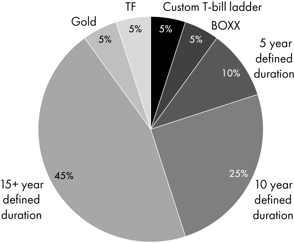
Here’s how our earlier example might look in a specific asset allocation:

• 0–3 year assets: 5% custom T-bill ladder over three-, six-, and 12-month bills. 5% BOXX (Alpha Architect 1-3 month T-Bills) for added tax efficiency.
• 3–7 year assets: 10% across 5 year defined duration instruments such as short-term bonds or multi-asset instruments with a shorter average defined duration.
• 7–15 year assets: 25% across 10 year defined duration instruments such as 7–10 year bonds, the Countercyclical Rebalancing Portfolio, 60/40, GFAP, Risk Parity, etc.
• 15+ year assets: 45% across assets with a 15+ year defined duration such as any all stock portfolio in this book or a blend of the Forward Cap Portfolio.
• Perpetual insurance: 10% diversified over gold, Trend Following and other insurance-like alternatives.

Figure 20.4: Defined Duration Portfolio

This blends a lot of the concepts we’ve discussed in this book, but adds a financial planning aspect in the asset-liability matching process that better aligns our portfolio with our actual financial plan.

DEFINED DURATION PORTFOLIO ANALYSIS

This is a uniquely financial planning-based portfolio so it’s hard to generalize about the performance since it will always be implemented in a personalized manner. That said, the strategy will end up looking like a custom bond ladder with additional five-, 10- and 15+ year target components. The five-year instrument should look roughly like a three- to five-year bond over time, the 10-year instrument should behave like the GFAP or Countercyclical Portfolio over time and the 15+ year instrument should track closely with a broad stock index over time.

The five-year instrument you utilize should tilt towards something more conservative as you have an inherently short time horizon here. This could be as simple as a mix of intermediate bonds, an aggregate bond index or even a conservative stock/bond blend. But it should be an inherently more bond-like instrument with greater emphasis on principal stability relative to purchasing power protection and/or growth.

Your 10-year instrument is going to be more balanced given the intermediate time horizon it’s designed to address. At this range, it’s not ideal to be 100% in stocks, but it’s also too long a horizon to rely solely on bonds. This is why blending an instrument with a balance of stocks and bonds can work nicely here. As I mentioned before, a 60/40 stock/bond instrument works out to a roughly 12-year instrument so that is a simple piece of the puzzle that can work for many investors. I prefer to throttle the stock market risk a bit by tilting the portfolio more towards bonds using the countercyclical rebalancing strategy.

Your 15+ year bucket is going to be aggressive and can include a single or many aggressive components. I typically like to tilt this bucket in a more growth and momentum-oriented fashion given the inherent riskiness of the allocation. This bucket is where we can take pure stock market risk or even tilt to something that is taking on more risk than the broader market.

And if you include the insurance component, the portfolio takes on a distinct profile compared to a traditional stock/bond ladder, as it allows you to layer in a variety of alternative assets.

In total you end up with a portfolio that looks like a bond ladder except instead of using only fixed income instruments, you’re diversified specifically across many different types of holdings.

In terms of performance, this is very specifically not a beat-the-market portfolio in its entirety. It is a financial planning-based portfolio that can be customized in any way necessary.

DEFINED DURATION PORTFOLIO PROS AND CONS

This is my personal favorite portfolio so we can’t be too critical, right? Wrong. Let’s dig into the bad news.

1. The Defined Duration Strategy is not a beat-the-market portfolio so it could test your patience. Further, it is designed to be very broadly diversified so there will always be parts of it that frustrate an investor.
2. The insurance component is optional and might not be applicable to everyone. Instruments like gold, managed futures, TIPS, or long-term T-bonds might not be necessary for all investors.
3. While this portfolio can be implemented using a DIY approach, it’s ultimately designed as a financial planning strategy. For that reason, it’s wise to either work with a financial advisor or build a solid DIY financial plan as the foundation.
4. The strategy ultimately ends up looking a lot like a value and momentum strategy where the shorter-duration instruments are tilted slightly to value (and quality) and the longer-duration instruments are tilted towards growth and momentum. This creates diversification, but will also create higher volatility in the long duration bucket that will test your patience at times.

And what about the good news?

1. This is a unique, planning-based asset allocation approach that prioritizes your actual expenses – rather than relying on vague risk profiling or beat-the-market strategies. Because it’s built using a framework of clearly defined temporal buckets aligned to specific financial needs, it creates a behaviorally robust portfolio – one that’s easier to stick with through market ups and downs.
2. The portfolio can be incredibly simple, almost as simple as the Three-Fund Portfolio, but much more customized and much more diversified.
3. The portfolio is low-cost, tax efficient, and highly diversified.

SUITORS FOR THE DEFINED DURATION STRATEGY

The Defined Duration Strategy is ideal for investors who value structure and seek greater certainty around their financial plan. While it can benefit anyone, it’s especially well-suited for those nearing or already in retirement – periods of life where the uncertainty around time and future expenses is often at its highest.

This approach could also be used in a simple format within retirement plans and 401(k)s for investors seeking a more disaggregated option relative to instruments like target date funds.

It’s also a great tool for financial advisors who are looking to give their clients more clarity around their financial plans.

If you have questions about the approach, feel free to shoot me a note. If you have criticisms, you know who to contact (not me).

FINAL THOUGHTS

You might be thinking we’re wrapping things up – but not quite yet. Hang in there; we’ve got a few more loose ends to tie up and some important ideas still worth exploring.

In the next chapter, we’ll take a look at a few additional strategies and asset classes that may be worth considering. You know, just in case you haven’t quite found what you’re looking for....